
This article was translated into English in my own way after listening to the presentation of voxel-based shadow processing research released by the Unity Spotlight team in 2019.
While living in China, I participated in the development of two mobile MMO Rpg( Fully Open World Mobile MMORPG ).
Real-time shadow handling is a very difficult optimization difficulty.
I didn’t use the latest technology, but I optimized it so that only a small amount of draw calls are consumed in one scene.
I call it Shadow Proxy volume.
I will introduce it in detail later.
However, that method does not guarantee consistency.
In addition, real-time shadows were processed using the Variable Shadow technique, which is a low-resolution shadow map, but achieves a visual improvement over the Unity default shadow algorithm.
The voxel-based shadowing technique is very interesting, so I will summarize and share the contents.
Thank you to the Unity Spotlight team.

Presentation: Kim Sung-Dae by Unity Spot-Light Team Graphics Programmer.

summary.
- Introduction to existing cases.
- Introduction of ideas.
- Implementation description and rendering.
- Results and performance.
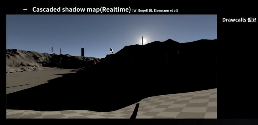
Typical cascade shadow method.
Although it has advantages, But it requires a number of draw calls.
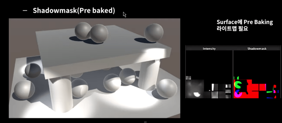
Shadow mask method.
It also need a pre-baked lightmap on the surface

Signed Distance Fields Shadows(Pre baked)
It can reach better quality shadows, but you also need a pre-baking lightmap on the surface.
The Voxelized Shadow method to be introduced today.
Since no UV is required, the same density and consistency can be guaranteed for the entire scene.

Since the shadow information has already been baked in the octree space, it doesn’t matter if you add a dynamic object
No additional shadowing required, even when using volumetric lighting.

Introduction of ideas.
– Shadow map voxelization.
–Expressed in SVO.
– Compressed with DAG structure.

I used the above scene for understanding.
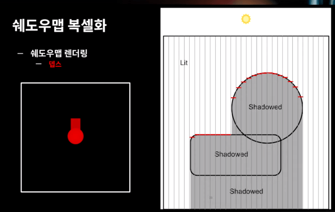
Red is the depth.
In a general shadow processing method, We can draw a shadow by determining whether or not it is shadowed using the depth as above.

When implementing the voxel shadow, I divided the space into a uniform grid and saved it.
At this time, it is saved in 0 or 1 format (binary 1 bit)

When Voxelized, 8GB capacity is required for 4K * 4K * 4K * 1bit.

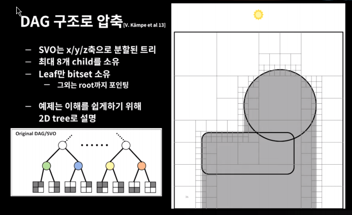
SVO structure is used because it is inefficient when using a uniform grid.

Only the outline part is processed.
Unnecessary Child is no longer composed.

Parents can own up to 8 children.

First, the leaf node owns the bit set.
Process the bit set according to the silhouette.
The upper node has only pointing and does not have separate data.
Pointing but using that information to infer correct data information

Optimized 8 GB to 3.8 Mega (1st stage)
It is not a structure that can be used only at the SVO level.

Before explaining the DAG structure, let’s first summarize the SVO steps.
Tree structure divided by xyz.
Up to 8 children.
Only leaf nodes own bit sets.
Other one use only pointing included root.
It examples are described in 2D structure for easy understanding.
It is actually an octree structure.
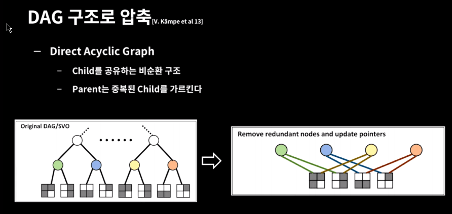
Brief description of the DAG structure.
有向无环图 Direct Acyclic Graph. https://en.wikipedia.org/wiki/Directed_acyclic_graph
Acyclic structure that shares the child.
Parent refers to the duplicated Child.
Looking at the picture above, you will see overlapping nodes.
It compresses in a way that shares these overlapping things.
The figure uses a two-dimensional graph for simplicity.
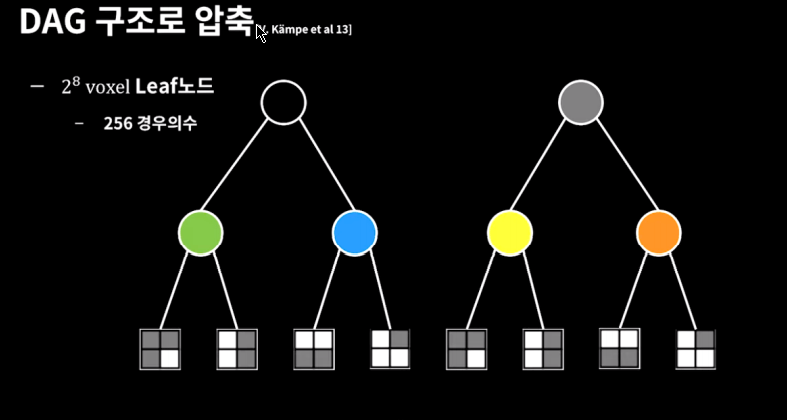
In this example, it is a voxel loop of 2 to the 8th power.
The total number of cases generates the number of 256 cases.
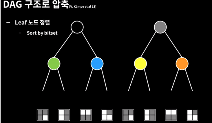
Leaf nodes have information about bit sets and can be sorted.
After sorting, search for duplicates by sorting by near ones.
Delete duplicates right away.
Re-update the parent node to complete the DAG phase of the leaf node.
Parent node alignment.
Search for duplicate nodes by sorting parent nodes.
The result after DAG processing is compressed, but the same result is output.
Compressible reason: binary data.
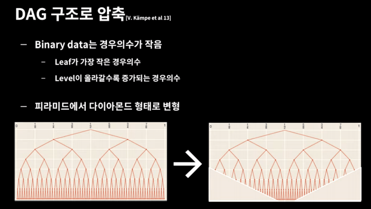
- Binary data has a small number of cases.
- Number of cases where Leaf is the smallest.
- The number of cases that increase as the level goes up.
- Transformation from pyramid form to diamond form.
See DAG paper.
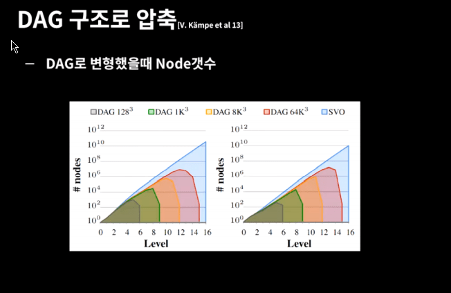
Compression ratio comparison.

First-order optimization from the first 8 gigabytes to 3.8 megabytes.
Optimized to 0.2 mega after DAG compression.

Implementation description and rendering.

Implementation description and rendering.
- SVO/DAG data structure.
- Build pipeline.
- SVO/DAG build.
- Rendering (tree navigation).

SVO/DAG Data Structure.
Save as UInt in Compute Buffer.
- Stride : 4
- Count : Variable
2*2*2 divided.
Node size is variable.
Implemented in Compute Shader.

- Node Header
- Unused:16bit.
- Childmask: 16bit.
- Childmask
- Use 2bit per child.
- 0x0001 : lit
- 0x0002 : shadowed
- 0x0003 : intersected
- Child exists.
- Child pointer#
- 32bit
- Stride index(not byte index)
There is a child pointer, which depends on how the child mask is structured, the size of the node varies.
If there is no child, only the header exists and ends.
The header is first 16 bits unused.
Child mask uses 16 bits.
Use 2 bits per child.
In the first case, the child receives the light.
In the second case, the child receives light.
In the third case, intersected, that is, to judge that it is not yet known.
Child pointers are stored in 32 bits.
Inside it has a stride (4 bytes) index.
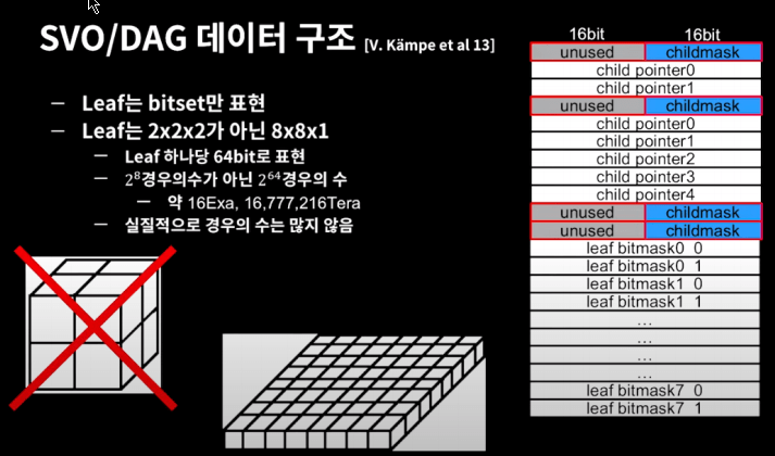
- Leaf expresses only bitset.
- Leaf is 8x8x1, not 2x2x2
- Expressed in 64 bits per Leaf.
- 264 cases, not 28 cases
- about 16Exa, 16,777,216 Tera
- In practice, there are not many number of cases.
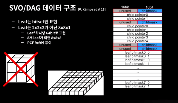
当它变成8叶子时,它是8x8x8
易于PCF 9×9。
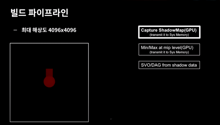
Build pipeline.

Built on CPU at the time of 2019.

Calculated on GPU in min max unit.
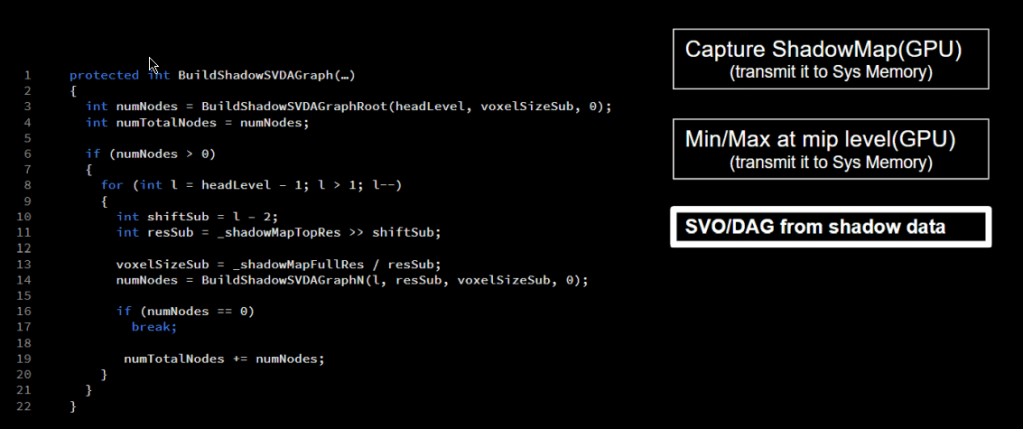
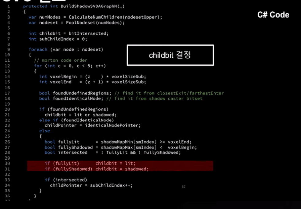
Simple code to help you understand.
Compression through the following method.

8K

16K

Create a root node.
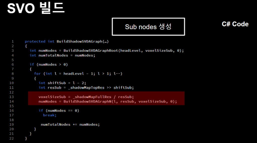
Sub node processing in more detail while looping.


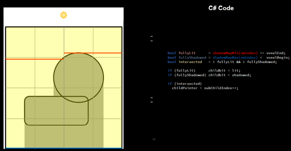
Voxel bounce and shadow mip-maps can be compared.
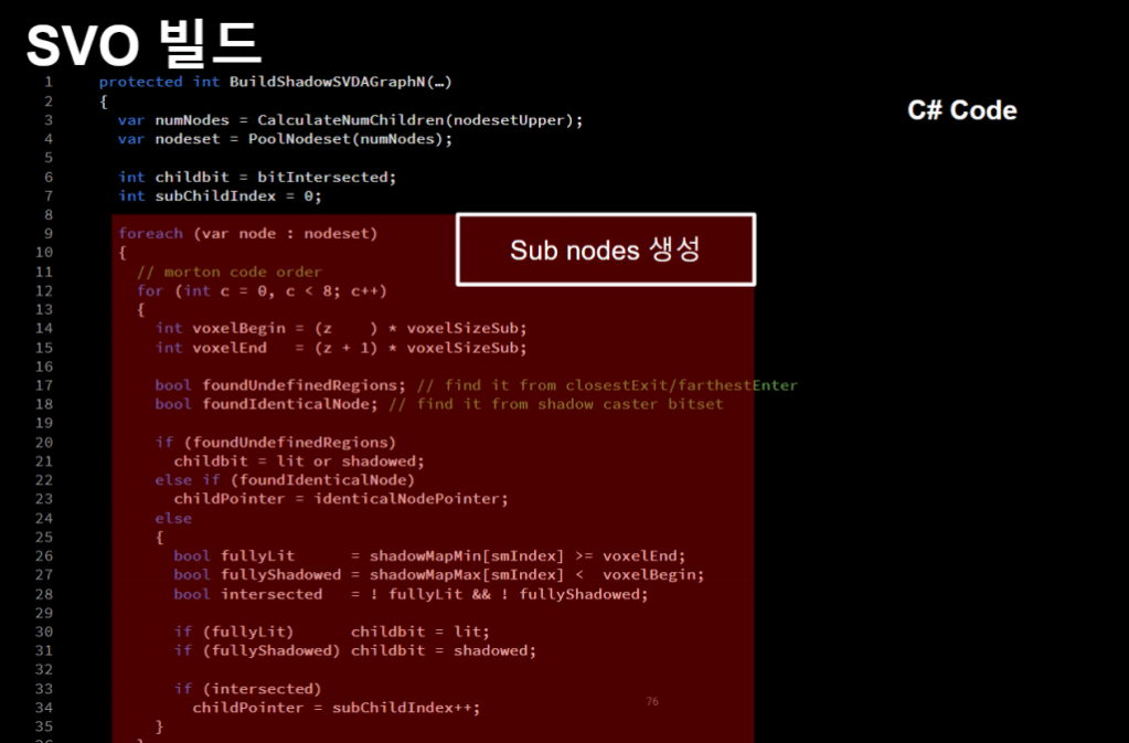
For each step, the CPU has a Min and Max value.
Voxel status can be determined.
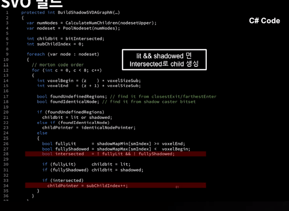
In the intersected state, a child pointer is added.
Discrimination loop in the child bitmask area that exists in the head node.
Visualization of the discrimination process.
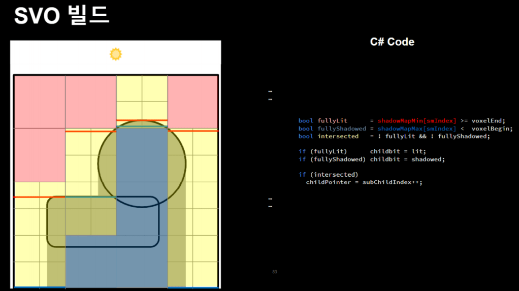


Up to this point, you can see that it is the SVO build, and the outer part is calculated intensively.

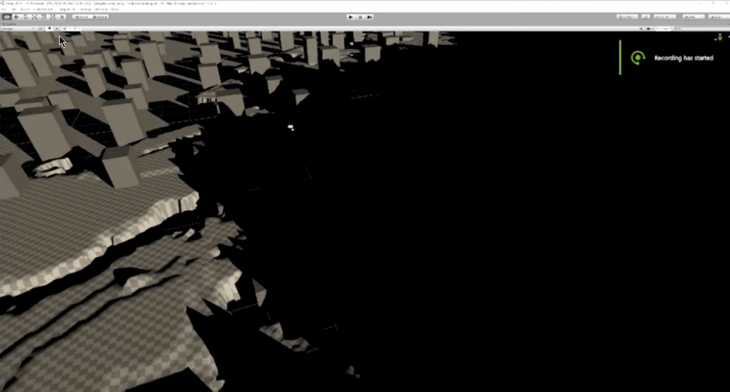
Rendering result.

VoxelDAG Shadow features.
3D data octree → Tree search.

Compute Shader consisting of hlsl.
Go down the loop while searching the tree.
Determine the state of the desired point.

Rendering (Tree searching)
Determine the child position to move by bit operation.
Convert P to UInt. (Assume that P is world space. )
- When the first spatial transformation of the world space point is performed, if it is converted to UInt according to the resolution, it is shown as bits.
- In the form of this bit, the bit indication that is replaced for each level immediately knows which child to go to.
- Separate conversion is not complicated.
World-Space → Light-Space
Position→ NDC → [0…Res]
Determine the position of the child to which position to go.

- Determine which voxel the Child is.
- Lit
- Shadowed
- Intersected
- if lit, then 1
- Else if shadowed, then 0
- Else keep going down.
Child mask set.
Heather Determines whether the child to go is in the light or not.
It is 1 when it receives light and 0 otherwise.
If it is not the two above, it will continue to descend on the loop.

- Lit or Shadowed ends the loop.
- If intersected, the next level is lowered.
- Get the child’s pointer.
- Loop through to the last level.
When it becomes status of intersected, it continues looping while moving to the next level.
If there is an intersection, the loop runs, otherwise the loop ends and returns.
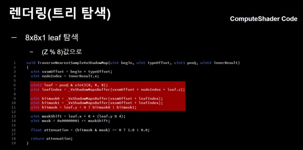
Leaf node search.
Searching used by different method.
Determines which leaf to jump to with the remaining value of Z.
For the sake of simplicity, we use near-list sampling (bilinear sampling, etc.)


Visualize and describe.
We defined it as Early Termination.
In the image chart, the left side is far from the silhouette area, so the loop ends quickly and is determined quickly.

This result is visualized by inserting all the information calculated at various angles into the compute buffer.
In general, when the shadow is baked, the dynamic object is processed so that it darkens slightly when the dynamic object is in the shadow area by using a Light-Probe.
However, since Voxelized Shadow has already baked the shadow information in the octree space, it has the advantage that the same shadow effect can be applied to the dynamic object and the draw call does not increase separately.

결과 및 성능 ( 2019년 개발 버전 기준 )

Compared size of memory consumption.
ShadowMap 16bit(Default shadow type) 4K(Distance) : 32Mega
VoxelShadow 4K(Distance): 1.6 Mega
ShadowMap 16bit(Default shadow type) 16K(Distance) : 512Mega
VoxelShadow 16K(Distance): 8.6 Mega
Optimization 1 and 2 will be provided as appendix files.


- Pros
- High resolution shadow lighting available.
- Static object shadow solution.
- Cast shadows on dynamic objects without additional draw-calls.
- Volume lighting support.
- one pass draw-call
- Cons
- Need Pre-computation
- Only tree searching.
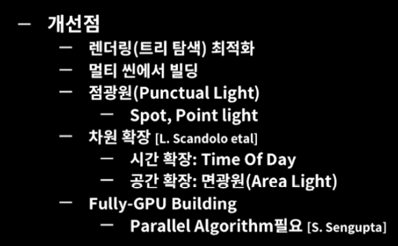
Future improvements.
- Optimization of rendering (tree navigation).
- Building in multi-scene
- Punctual light
- Spot, Point light
- Dimensional expansion (consistent characteristics over time are compressed into one)
- http://graphics.tudelft.nl/Publications-new/2016/SBE16a/SBE16a.pdf
- Time of Day
- Space expansion: Area Light
- Fully-GPU building
- Parallel algorithm required.
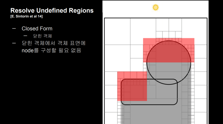
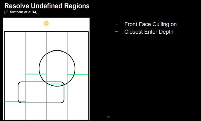
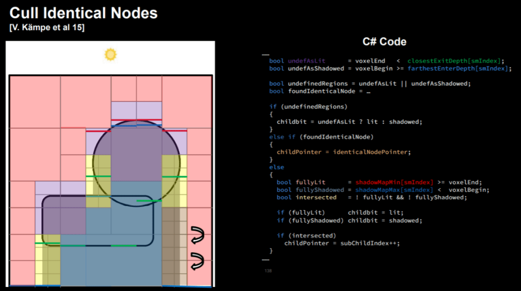
- Closed Form
- No need to construct a Node on the object surface in a closed object.

- Advantages
- Node quantity reduction
- Building time reduction
- Performance increase
- Shadowing result is the same
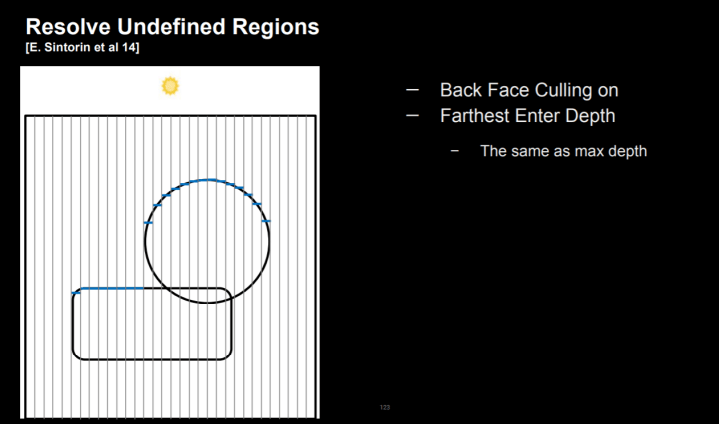
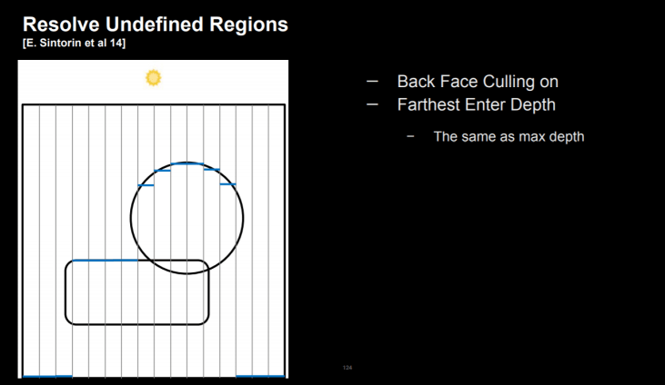
- Requires 2 shadow maps
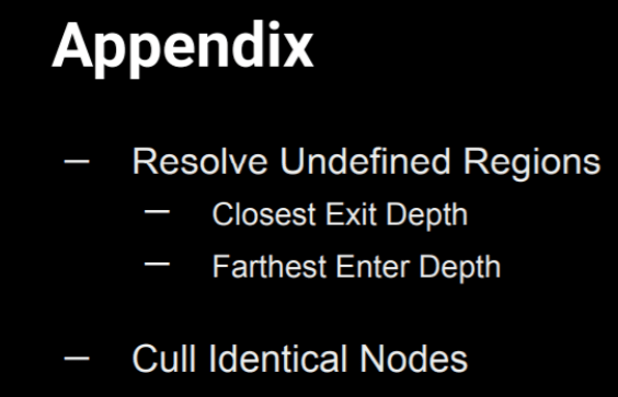
- Front/Back Face Culling rendering
- Farthest Exit Depth
- By Back Face Culling
- Closest Enter Depth
- By Front Face Culling


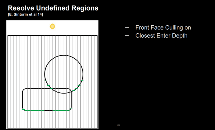
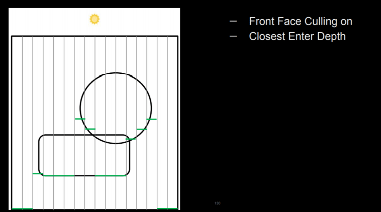

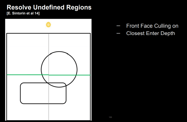

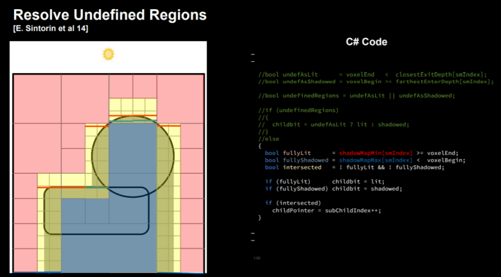


- The depth value is the shadow caster.
- There is a possibility of overlapping because there is no shadow caster in the node.
- If the previous Node exists, copy it.
- You only need to bring the Pointer.
- No more Subtree configuration required.
End of contents.

댓글 남기기